Self Organizing Maps
- May 21, 2017
- 5 min read
All code and files discussed in this tutorial can be found at GitHub.
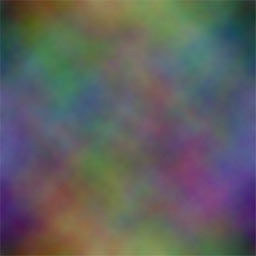
Before going further we will understand the core algorithm well. To understand this algorithm I have taken an image as an example.

Figure. 1 Example image taken to illustrate SOM algorithm.
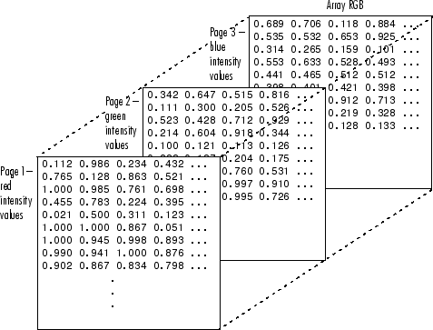
This image is made up of various colors. Actually an image is a 3D dataset having R, G, B array at the back.

Figure.2 Image to illustrate RGB layers of image (Image curtsy Mathworks)
As we see this image, it is having various colors. Visual color is a visible part of this image. The values behind this image is hidden part of this image. Hidden data is actually responsible for visual colors. It is very much clear from the above figure that each image is made up of 3D array of intensities of blue green and red. If such 4D data-set was provided then we would not be able to see it as we see this image. particular cluster. Such dimensions (here RGB) is known as weights in SOM. As I have taken image as an example, we can visualize form beginning and can recorded the progress of algorithm visually. It is absolutely not necessary to have visual data from beginning. We can have 100 dimensional data and hence 100 such weights are ultimately responsible for classification of that single data point in to any suitable cluster.
Main Algorithm

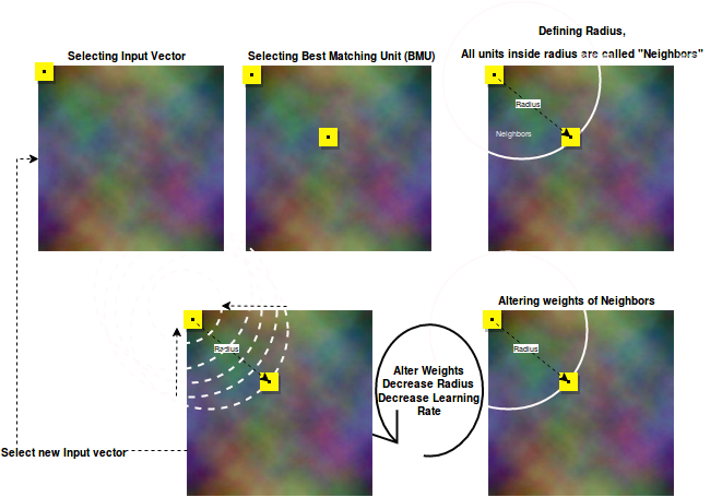
Figure 3. Flowchart explaining Self Organizing Map algorithm.
Self Organizing Map Algorithm involves following steps:
In given multidimensional data-set, select a point called input vector,
Find a another point in data-set called BEST MATCHING UNIT (BMU), using euclidean distance.
Define a radius between input vector and BMU, all units in this radius are called “Neighbors”
Alter weights of neighbors using learning rate
Decrease learning rate and radius exponentially
Alter weights of neighbors using learning rate
Repeat Steps 4 5 6 for specified number of iteration
Now, we will see each step in detail STEP – 1. Selecting Input vector.
We have a 256*256 pixel image. Virtually any point can be the Input vector. Here I have taken (0,0) the first pixel as starting point.
STEP - 2 Finding best matching unit.
Best matching unit is found out by using euclidean distance, Euclidean distance of all units (pixel) w.r.t. Input vector is measured. And the one which is at least euclidean distance is selected as BMU. Lets say e.g. we got point at (102,105) as BMU.We can call these input vector as well as BMU as lattice also as per formal SOM naming convention.
STEP – 3 Defining Neighbors
vector.An imaginary circle is taken keeping radius equal to distance between Input vector and BMU and Input vector as center of circle. All those units which lies in this circle are called neighbors. Neighbors are the units, whose weight will be altered in next iteration to make them similar to Input
STEP – 4 Altering Weights
For altering weights following step are followed2) For the selected neighbor new weight are calculated as follow.Selected neighbor will be updated with new weights1) Each neighbor is selected turn by turn.In above described way weights of all neighbor are changed in given radius.newweight = Weights of Selected Neighbor + (learning rate * difference of weight of input vector and weights of Selected Neighbor)
STEP – 5 Updating Radius and Learning Rate
new learning rate = initial Learning Rate * (math.exp(-time Or Iterations / rateOfDecay)) Once step-3 is completed as described, the radius of circle and learning rate are exponentially decreased. new radius = initialRadius * (math.exp(-timeOrIterations / rateOfDecay))Radius is decreased as follow : Learning rate is decreased as follow :

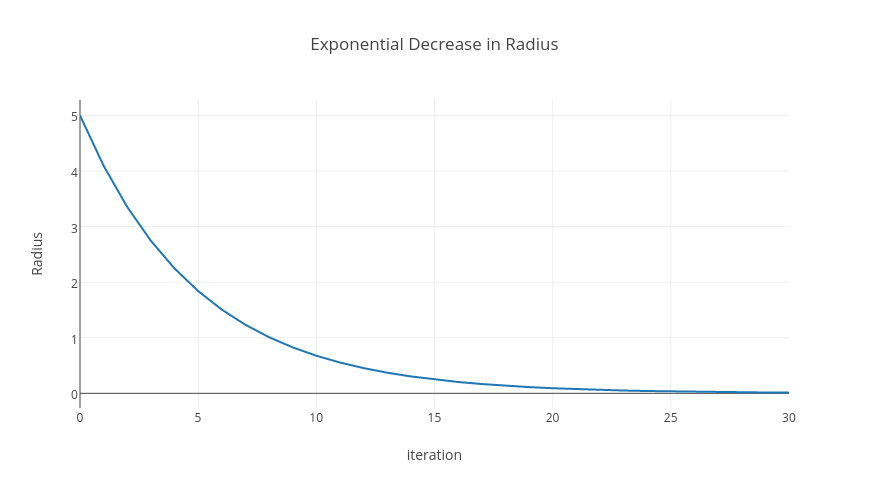
Figure 4. Plot to explain progress of Exponential Function. refer this worksheet to understand more about exponential functions.
Above given worksheet and picture is worth 100 words. You can clearly see the change in Radius exponentially. Such exponential decrease occur in learning rate too.
STEP – 6 Iteration
Once learning rate and radius are decreased steps 3,4,5 are performed for the number of iteration specified. Here in this implementation I have specified it as 10.
STEP – 7 Selection Next Input Vector
Earlier we have started with pixel (0,0) as input vector now we will move to (0,1) as input vector and perform all steps 2,3,4,5,6 again and again until we cover entire length and breadth of the image.
This is all about the entire algorithm. Once have clear picture in mind, we are now moving to actual implementation. We will understand each function first and then overall flow of algorithm as discussed.
LoadImage in the form of numpy array :
def load_image(infilename): """ will load image from the file :param infilename: filename :return: numpy array of image """ img = ndimage.imread(infilename) data = np.asarray(img, dtype="int32") resized = data.reshape(data.shape[2], data.shape[0], data.shape[1]) return resized
To get RGB value for given pixel
def getRGBForPixel(imageArray, i, j): """ for a particular pixel, it return RGB value :param imageArray: :param i: :param j: :return: """ return imageArray[i, j]
Set RGB value for pixel def setRGBforPixel(imageData, i, j, RGBValue):
""" for a particular pixel, it set RGB value :param imageArray: :param i: :param j: :return: imageArray """ imageData[i, j] = tuple(RGBValue) return imageData
To get Euclidean distance between two pixel (here called as lattice). e.g. we have taken (0,0) as input vector and (102,105) as BMU. Euclidean distance between such two pixels is measured by below given function. def findEucledeanDistanceBetweeenLattice(lattice1, lattice2):
""" if two point on 2d surface are given, it will return distance between two points :param lattice1: list [x,y] :param lattice2: list [x1,y1] :return: """ return math.sqrt(math.pow(lattice1[0] - lattice2[0], 2) + math.pow(lattice1[1] - lattice2[1], 2))
findNeighbors will find all neighbors between input vector and BMU
def findNeighbours(BMU, Radius, imageData, imageObject): """ If best matching unit (BMU) is found, it will find neighbours in given radius :param BMU: x y axis for winner node :param Radius: :param imageArray: :return: loacation of all pixel in 2-D plane [[1,2],[3,2],[4,2],....] """ width = imageObject.size[0] height = imageObject.size[1] neighbors = [] for i in range(0, height): for j in range(0, width): if findEucledeanDistanceBetweeenLattice(BMU, [i, j]) < Radius: neighbors.append([i, j]) return neighbors
findBMU - Finds Best matching unit for givan input vector specifiied by location
def findBMU(inputVectorI, inputVectorJ, imageData, imageObject): """ will find best matching unit for given inputVectorI and inputVectorJ :param inputVectorI: x :param inputVectorJ: y :param imageArray: :return: return x1 and y1 coordinates for BMU """ imageDataArray = PIL2array(imageObject) # print imageData, imageObject.size
minDistance = 9999999 width = imageObject.size[0] height = imageObject.size[1] minI = width + 1 minJ = height + 1 inputVector = getRGBForPixel(imageData, inputVectorI, inputVectorJ) for i in range(0, height): for j in range(0, width): R, G, B = getRGBForPixel(imageData, i, j) # print R,G,B distance = math.pow(inputVector[0] - R, 2) + math.pow(inputVector[1] - G, 2) + math.pow(inputVector[2] - B, 2) if (distance < minDistance and i != inputVectorI and j != inputVectorJ): minI = i minJ = j minDistance = distance break return minI, minJ
Calculate decay in Learning Rate and Radius
def decayRadius(initialRadius, timeOrIterations): """ will perform exponential decay of given radius :param initialRadius: radius at time t0 :param timeOrIterations: iteration number :return: """ rateOfDecay = 5 # MORE THE RATE MORE WILL BE THE TIME TAKEN TO REACH 0 return initialRadius * (math.exp(-timeOrIterations / rateOfDecay))
def decayLearningrate(initialLearningRate, timeOrIterations): """ will perform exponential decay of given radius :param initialRadius: radius at time t0 :param timeOrIterations: iteration number :return: """ rateOfDecay = 5 # MORE THE RATE MORE WILL BE THE TIME TAKEN TO REACH 0 return initialLearningRate * (math.exp(-timeOrIterations / rateOfDecay))
Updating weights of given neighbor. neighbor’s location in image is specified by co-ordinate (i,j).
def updateWeights(weightAtGivenNeighbour, inputVectorWeight, learningRate): """ will update weight and will return new weights, weights are basically RGB color of the image :param weightAtGivenNeighbour: RGB :param inputVectorWeight: RGB :return: """ newWeights = [] for eachweightNo in range(0, len(weightAtGivenNeighbour)): newweight = weightAtGivenNeighbour[eachweightNo] + (learningRate * (inputVectorWeight[eachweightNo] - weightAtGivenNeighbour[eachweightNo])) newWeights.append(int(newweight)) return newWeights
I have recorded progress of the algorithm at every 100 iterations. You may see it clearly in this folder. how at the end SOM separates all colors in different part of image. similarly we can use this algorithm to view multidimensional data into separate clusters in 2D image like representation.


Comments