Multivariate Adaptive Regression Splines (MARS), PART - 1
- Apr 9, 2017
- 6 min read
You may refer this literature for mathematical explanation of below implemented algorithm 1) http://www.lans.ece.utexas.edu/courses/ee380l_ese/2013/mars.pdf
2) https://www.assct.com.au/media/pdfs/Ag%2022%20Everingham%20and%20Sexton.pdf
All codes discussed here can be found at my Github repository.
For effective learning I suggest, you to calmly go through the explanation given below, run the same code from Github and then read mathematical explanation from above given links.
Code compatibility : Python 2.7 Only
Often it is found that due to changing requirement with change in package versions code fails to run. I have added file named requirement.txt file to GitHub, which shows all packages with version present in my system when I executed this code. This will help in replicating working environment and debugging.
To get this code running execute Introduction.py file as given in GitHub repository.
Before going to mathematical formulation lets start with one example, that will make you understand why this technique exists.
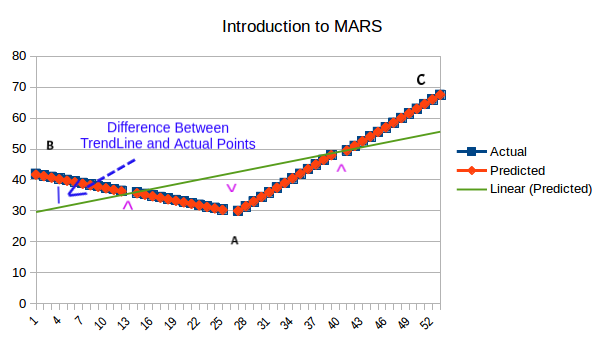
Fig 1. Introduction to MARS
As shown in Fig 1. we have data distribution as shown in blue and we want have found out trend-line as indicated by green line. This green line Doesn't make justice when it comes to overall generalisation. When one want to make prediction near point A or B or C, it will be predicted with highest error. So having one line trend-line for such data is not sufficient.
Assume if we have multi-part trend-line as shown on Orange then it perfectly represents data, and all prediction made from such trend-line will be least erroneous.
MARS is all about getting personalised trend-lines for different fragment of data so that data with wide spread, larger ups and downs can be predicted well.
MARS at at once is little hard to understand, So I Have developed it incrementally.
A. Introduction with synthetic data.
B. Moving ahead with real data ( Explained as - PART - 2)
C. Application of Forward Run [A sub part of MARS] ( Explained as - PART - 2)
A. Introduction with synthetic data
Fig. 1, is made up from synthetic data. The same data we will take throughout entire subtopic to understand primitive implementation part of MARS.
We will use three functions to implement MARS in this section.
We will be having data as shown below :
inputData = [[1, 42], [2, 41.5], [3, 41], [4, 40.5], [5, 40], [6, 39.5], [7, 39], [8, 38.5], [9, 38], [10, 37.5], [11, 37], [12, 36.5], [13, 36], [14, 35.5], [15, 35], [16, 34.5], [17, 34], [18, 33.5], [19, 33], [20, 32.5], [21, 32], [22, 31.5], [23, 31], [24, 30.5], [25, 30], [26, 31.5], [27, 33], [28, 34.5], [29, 36], [30, 37.5], [31, 39], [32, 40.5], [33, 42], [34, 43.5], [35, 45], [36, 46.5], [37, 48], [38, 49.5], [39, 51], [40, 52.5], [41, 54], [42, 55.5], [43, 57], [44, 58.5], [45, 60], [46, 61.5], [47, 63], [48, 64.5], [49, 66], [50, 67.5]]
There are 50 data points, each with X and Y in pair.
All points are indicated by ^ are called breakpoints, In above given example total 4 trend-line exists. Next we will see how to calculate break points. To make different trend-line for different section of data, it is very much essential to separate fragments of data which are separate from each other or to clump like continuous fragments to-gather.
1) Calculate trend line for entire set of data.
2) Find positive difference between points on Trend-line and actual points as shown in Fig. 2
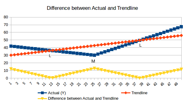
Fig. 2 Difference between Actual and Trend-line
Positive difference between Actual points and points on Trend-line is shown in yellow
3) Find out points where there is abrupt change in difference, it may result in two way
where point on Trend-line and actual line meets as shown by (L) in Fig. 2
where point on Trend-line and actual line at farthest (M) in Fig. 2
These break points then divide all data points into different continuous fragments of in the graph. Each fragment will have its own regression equation (here linear regression equation). Here in above shown graph we got four fragments [1 - 13] [14 - 25] [26 - 37] [38 - 50].
As we are clear about theory part, lets see implementation part. I promise you Its super easy :-
1) Calculate trend line for entire set of data.
Its super easy and we will be using the same function as used in Introduction To Regression.
2) To find positive difference between points on Trend-line and actual points as shown we will use function - simple MARS.
def simpleMARS(inputData): """ This function only finds trend-line and shows trendline for each fragment this is without forward run, where many small fragment exists :return: """ xArray = [] yArray = []
# separating data in to X and Y """ if data is something like [[1,0],[2,5],[3,6],[8,7],[10,8]] then xArray and yArray would look like this xArray = [1,2,3,8,10] yArray = [0,5,6,7,8] """ for eachXYPAir in inputData: x = eachXYPAir[0] y = eachXYPAir[1] xArray.append(x) yArray.append(y) # getting trend line for the entire data m, b = findTrendline(xArray, yArray)
difference = [] # will store difference between actual value of Y and Ypredicted given X (Y derieved from trendline) yArray = []
for eachXYPAir in inputData: # separating data in to X and Y x = eachXYPAir[0] y = eachXYPAir[1] # getting Ypredicted using previously calculated b (regression coefficient) and m (slop). # Ytrend will be the trend-line as shown in graph Ytrend = m * x + b # finding derived value of Y called as Ytrend (y derieved from trendline) from so found m and b in previous code block yArray.append(y) # difference are differences between Ytrend and Yactual points in YArray difference.append(abs(y - Ytrend)) # print y , Ytrend , abs(y-Ytrend) # lets print and see how we will define breakpoints here """ Breakpoints here are the point which separates group of data having similar slop, locally called fragments
Once Ypredicted (points on trend-line) and Y actual gives positive difference, The difference is passed to findBreakPoints function to get breakpoints.
""" breakPoints = findBreakPoints(difference) # getting breakpoint using findBreakPoints function [[1 ,2,3..,11,12,13] [14,15,16...23,24,25],[],[]]
for eachFragment in breakPoints: # break points will be like this # print eachFragment, # you may try this
# Getting x and yActual for the given Fragment range xFragment = xArray[eachFragment[0] - 1:eachFragment[-1]] yFragment = yArray[eachFragment[0] - 1:eachFragment[-1]]
# finding trendline for the given Fragment range, individual trend-line for each one m, b = findTrendline(xFragment, yFragment)
# Getting yTrend for the given Fragment range yDerived = [xArray[j - 1] * m + b for j in range(eachFragment[0], eachFragment[-1] + 1)]
# printing value of yactual and yTrend for printing for i in range(0, len(xFragment)): print yFragment[i], yDerived[i] print ""
3) Find out points where there is abrupt change in difference, to detect breakpoints
To understand functioning of findBreakPoints , please have a look at Fig. 3 and go through comments in the code given below.
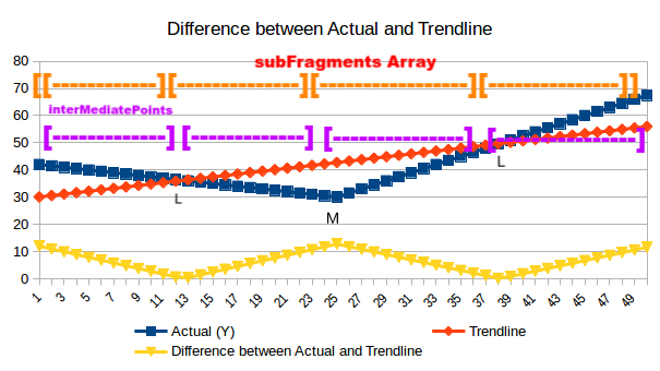
Fig 3. Understanding functioning of findBreakPoints function.
def findBreakPoints(difference): """ find breakpoints for allocation of different slop (m) and coefficient (b) to each fragment :param difference: is the array which shows what is the difference between current point and the same point on trend-line :return: subFragments, also referred as brekpoints """ subFragments = [] # print len(difference) lastPoint = 0 interMediatePoints = [] for i in range(1, len(difference) - 1): # iterating through array having difference between trend-line and actual points interMediatePoints.append(i)
"""
interMediatePoints is an array used to store intermediate points, once any of the below given if condition becomes true all points appended in interMediatePoints will be submitted to subFragments array as an fragments.
""" if difference[i - 1] > difference[i] < difference[i + 1]: """if difference at given point i is lesser than its surrounding points : [i+1] and [i-1] , it will be defined as breakpoint this will be a crest in local region \/ """ lastPoint = i subFragments.append(interMediatePoints) interMediatePoints = [] # print "low Diffrernce point Identified", i + 1 if difference[i - 1] < difference[i] > difference[i + 1]: """if difference at given point i is higher than its surrounding points: : [i+1] and [i-1], it will be defined as breakpoint this will be a crest in local region \/ """ lastPoint = i subFragments.append(interMediatePoints) interMediatePoints = [] # print "High Difference point Identified", i + 1
# processing last fragment
"""
Last fragment (/) of the data point [\__/\/ ] do not get captured in above written "if conditions" so processing last fragment separately.
""" subFragments.append([j for j in range(lastPoint + 1, len(difference) + 1)]) return subFragments
This is all about simple approach to understand MARS , In up coming part - 2 of the tutorial we will apply same function to the real data , and further develop the approach.


Comments