What is Stochastic Gradient Descent (SGD)
- Apr 2, 2017
- 6 min read
You may refer this literature for mathematical explanation of below implemented algorithm 1) http://joyceho.github.io/cs584_s16/slides/sgd-3.pdf
2) http://leon.bottou.org/publications/pdf/compstat-2010.pdf
All codes discussed here can be found at my Github repository
For effective learning I suggest, you to calmly go through the explanation given below, run the same code from Github and then read mathematical explanation from above given links.
Code compatibility : Python 2.7 Only
To get this code running run stochasticGradient.py file as given in GitHub repository
Preferably the title would be Stochastic Gradient Descent (SGD) without Much Mathematics.
Let get known to much talked error minimization algorithm. If you will search on internet for the same, I ma sure you will get frighten by looking at mathematical equations. Don't worry I will explain more practically, less Mathematically.
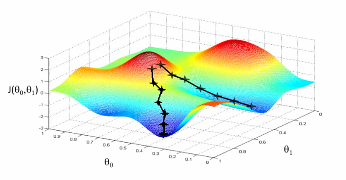
Stochastic gradient descent (often shortened in SGD), also known as incremental gradient descent. Non technically we can say that it is the technique to decrease error gradually. before moving further it is very essential to understand what actually a minimization algorithm is ?
We will not go straight forward to mathematical form of the algorithm, we will first take one example and will see how it actually works.
One question? when error happens? when we try to predict on the basis information we possess. right? We usually learn from such errors and better perform next time on the same task.
Similar to out learning process we have following component in out mathematical design to understand.
Input data
Desired output
Coefficient [can be taken similar to memory, which stores learning]
SGD to minimize error
Let take simplistic example of AND gate to understand SGD. SGD truth table look likes this. If both input a and b is same the output is 1 else 0. where input is known as X and output is known as Y.
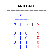
Figure 1. XOR gate truth table
Here our goal is to make machine learn, if input X is provided then based on previous learning machine shold be able to provide appropriate output Y.
As we have learned in previous blog post - Introduction to regression, we can apply regression here also.
For single input value - Y = βo +βax
For double input value - Y =β0 + βaXa + βbXb
where,
βo is an independent regression coefficient
βa + βb are coefficient for input Xa and Xb Respectively.
Xa and Xb are inputs.
Now lets start actual implementation of SGD. We have following units in our implemenation.
1) Data - AND GATE
2) Predict - used to predict on data using regression algorithm as discussed. It takes two inputs.
a) Data [[1,1]] , (only X part)
b)Previously learned coefficients and slops and predicts on given data.
3) SGD - used for to minimize errors and takes three 3 inputs
a) Data [[1,1,1],[01,1,0],[1,0,0],[0,0,1]] , whole data X and Y
b) learning rate (η) - Its is a value greater than 0 and lesser than or equal to 1 [ 0< η >=1]
c) Epochs - Number of time the same data to be given to the machine learning algorithm so that it can learn.
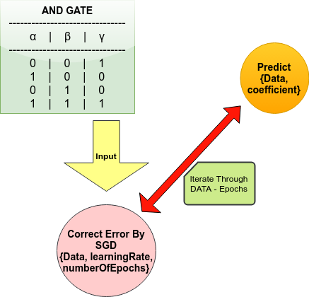
Figure 2. Flow chart to explain working of Stochastic gradient descent.
Input to SGD will be [[0,1,0],[1,1,1],[1,0,0],[0,0,1]]. where in each row [0,1,0]; initial two 0,1 inputs also called X and last one 0 is output called Y as shown in figure 1.
Lets understand Predict function first
Predict takes two inputs:
a) Data [[1,1]] , (only X part)
b)Previously learned coefficients (β0, βa, βb)
def predict(Xrow, coefficients): """ for prediction based on given row and coefficients :param Xrow: [1,0,0] where last element in a row remains Y [so called actual value y-actual] :param coefficients: [0.155,-0.2555,0.5456] Random initialization :return: Ypredicted
This function will return coefficient as it is real thing we get after training coefficient can be actually compared with memory from learning and be applied for further predictions """ """ Ypredicted = b0 + BaXa + BbXb Ypredicted = coefficients[0] - will take bo in to Ypredicted Ypredicted += Xrow[i] * coefficients[i + 1] - Ba and Bb are multiplies to Xa and Xb gives BaXa + BbXb """ Ypredicted = coefficients[0] for i in range(len(Xrow) - 1): Ypredicted += Xrow[i] * coefficients[i + 1] return Ypredicted # Ypredicted is return back
Now we are clear about predict part, lets learn what is happening in SGD function
SGD - takes three 3 inputs
a) Data [[1,1,1],[01,1,0],[1,0,0],[0,0,1]] , whole data X and Y
b) learning rate(η) - Its is a value greater than 0 and lesser than or equal to 1 [ 0< η >=1]
c) Epochs - Number of time the same data to be given to the machine learning algorithm so that it can learn.
def SGD(dataset, learningRate, numberOfEpoches): """
:param trainDataset: :param learningRate: :param numberOfEpoches: :return: updated coefficient array """
"""
we will be having one extra coefficient as per the equation discussed. For each column in train dataset we will be having one coefficient. if training dataset having 2 column per row then coefficient array will be something like this [0.0, 0.0, 0.0,] """ coefficient = [0.1 for i in range for epoch in range(numberOfEpoches): # iterate for number of epochs """ for each epoch repeat this operations """ squaredError = 0 # to keep eye over all cumulative change in error from first epoch to last epoch for row in dataset: """ for each row calculate following things where each row will be like this [1,0,1]==> where last element in a row remains Y [so called actual value y-actual] """ Ypredicted = predict(row, coefficient) # call predict, predict will work with given row and coefficient for prediction error = row[-1] - Ypredicted # row[-1] is last element of row, can be considered as Yactual; Yactual - Ypredicted gives error in prediction "Updating squared error for each iteration" squaredError += error ** 2 """
In order to make learning, we should learn from our errorhere we will use stochastic gradient as a optimization function SGD for each coefficient [b0,b1,b1,.....] can be formalized as :
coef[i+1] = coef[i+1] + learningRate * error * Ypredicted(1.0 - Ypredicted)* X[i]
For a row containing elements [xa, xb], coefficient [ ba, bb] where each coefficient belongs to each element in a row e.g. ba for Xa, bb for xb and so on.. As coefficient[i] here is equal to bo, e.g. row element independent, we will update it separately. """ coefficient[0] = coefficient[0] + learningRate * error * Ypredicted * (1 + Ypredicted) # calculating update for independent coefficient [b0] for i in range(len(row) - 1): # calculating update for all other coefficient [b1 and b2] coefficient[i + 1] = coefficient[i + 1] + learningRate * error * Ypredicted * (1.0 - Ypredicted) * row[i]
""" lets print everything as to know whether or not the error is really decreasing or not """ print " Epoch : ", epoch, " | squared Error : ", squaredError # will print squared error for each epoch return coefficient # will return coefficients, here coefficient are equivalent to model memory. using these we can predict on unknown samples
data = [[1,1,1],[0,1,0],[1,0,0],[0,0,0]] stochastic_gradient(data,.1,250)
I have explained entire procedure through comments in the code. If you are still unclear, get your hands dirty form my GITHUB repo, print confusing things and get your doubt clear. You may also prefer to comment in the blog post.
After running above code you will gate output something like this
Epoch : 0 , squared Error : 0.616480008695 Epoch : 1 , squared Error : 0.598279511475 Epoch : 2 , squared Error : 0.584645976545 Epoch : 3 , squared Error : 0.574658674109
.
.
.
.
Epoch : 249 , squared Error : 0.41588655655
After printing squared error in Microsoft Excel you will get following graph:
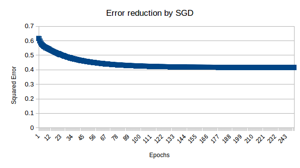
Now the big question here is, if algorithm is learning then why it stopped with constant error 0.4? . Ideally error should go near 0.0.
This phenomena is called learning insufficiency. We have total four combination to learn and we have 3 memory unit in equation. beside this we are using linear equation so it is very much possible that it is not able to learn everything.
To see the same in action. I have implemented entire algorithm in Microsoft Excel. where i have applied the same algorithm with SGD and I am getting similar results.
The excel sheet we are going to discuss is present on my GITHUB repository.
Here I have modeled in stochastic gradient in Excel sheet and perfectly depict the same result we have produced through python. Have a keen look at each variable and try to change learning rate from 0.1 to 0.11 you will see visual difference in the error.
We will see about learning insufficiency in further detail practically when I will start tutorial about neural networks.


Comments