ConvNet - Image Classification
- Nov 10, 2016
- 6 min read
Everything discussed under this tutorial including working code, pre-trained machine learning model is available on my GITHUB repository .
Often it is found that due to changing requirement with change in package versions code fails to run. I have added file named requirement.txt file to GitHub, which shows all packages with version present in my system when I executed this code. This will help in replicating working environment and debugging.
Code Compatibility : python 2.7 , tested on ubuntu 16.04 with theano as backend
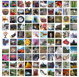
Figure. 1 Cifar Data-set
When It comes to image classification, Convolution Neural Network (ConvNet) are the best. ConvNets are designed for processing Images. ConvNets are being extensively used for image classification, image recognition, image tagging and deep dreaming.
In present blog we will use ConvNet for image classification. "Great usage comes with great Requirement" ; training a model using ConvNet is computationally intensive so we will be using GPU for the same.
I will be using AWS GPU with 3000+ core for the present tutorial. You may use normal machine with i3/ i5 CPU and 4 gb ram for this tutorial. I have tested and it works well on CPU too.
The CIFAR-10 data-set consists of 60000 32x32 colour images in 10 classes, with 6000 images per class. There are 50000 training images and 10000 test images. The data-set is divided into five training batches and one test batch, each with 10000 images. The test batch contains exactly 1000 randomly-selected images from each class. The training batches contain the remaining images in random order, but some training batches may contain more images from one class than another. Between them, the training batches contain exactly 5000 images from each class. We will be utilizing cifar image data-set.
The CIFAR-100 dataset
This data-set is just like the CIFAR-10, except it has 100 classes containing 600 images each. There are 500 training images and 100 testing images per class. The 100 classes in the CIFAR-100 are grouped into 20 superclasses. Each image comes with a "fine" label (the class to which it belongs) and a "coarse" label (the superclass to which it belongs).Here is the list of classes in the CIFAR-100:

Figure. 2 Superclass and Classes in cifar data-set.
[more the complexity greater the fun !!] We will be utilizing cifar-100 data-set
Lets code it then!!
Step 1. Importing required libraries
from __future__ import print_function
from keras.datasets import cifar100
from keras.preprocessing.image import ImageDataGenerator
from keras.models import Sequential
from keras.layers import Dense, Dropout, Activation, Flatten
from keras.layers import Convolution2D, MaxPooling2D
from keras.optimizers import SGD
from keras.utils import np_utils
from matplotlib import pyplot
from scipy.misc import toimage
%matplotlib inline
Step 2. Importing cifar100 data-set
Keras provide simple and easy way to import cifar-100 data-set for example use purpose.
We ill use the same:
(X_train, y_train), (X_test, y_test) = cifar100.load_data()
by default data-set is spitted in to test and train. Train data is having 50,000 samples and test data is having 10000 samples.
# lets print data size of all four section print ("X_train Size: ", len(X_train)," y_train Size :" ,len(y_train)," X_test Size : ",len(X_test)," y_testSize : ",len(y_test))
you will get following output :
X_train Size: 50000 y_train Size : 50000 X_test Size : 10000 y_testSize : 10000
You may wonder what is there in image actually, what image is made up of ?? Each image is made up of three layers RGB [Red Green Blue] each element can go from 0 to 255 in 8 bit image '
If you will hit X_train[0] then it will show RGB values for for the first image.
array([[[255, 255, 255, ..., 195, 212, 182], [255, 254, 254, ..., 170, 161, 146], [255, 254, 255, ..., 189, 166, 121], ..., [148, 142, 140, ..., 30, 65, 76], [122, 120, 126, ..., 22, 97, 141], [ 87, 88, 101, ..., 34, 105, 138]],
[[255, 255, 255, ..., 205, 224, 194], [255, 254, 254, ..., 176, 168, 154], [255, 254, 255, ..., 199, 178, 133], ..., [185, 182, 179, ..., 17, 62, 77], [157, 155, 160, ..., 16, 112, 161], [122, 122, 134, ..., 36, 133, 173]],
[[255, 255, 255, ..., 193, 204, 167], [255, 254, 254, ..., 150, 130, 113], [255, 254, 255, ..., 169, 130, 87], ..., [ 79, 57, 60, ..., 1, 15, 20], [ 66, 58, 71, ..., 3, 56, 87], [ 41, 39, 56, ..., 10, 59, 79]]], dtype=uint8)
Step 3. Visualize
% lets visualize first 3 images , matplotlib inline declaration in ipython help to visualise images Inline. All images are 32 * 32 in dimension.
pyplot.imshow(toimage(X_train[0])) #showing first image
pyplot.show()
pyplot.imshow(toimage(X_train[1])) #showing second image
pyplot.show()
pyplot.imshow(toimage(X_train[2])) #showing third image
pyplot.show()
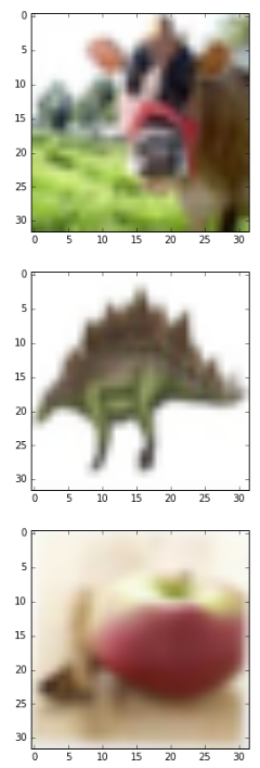
Figure 3. Few Images from Cifar data-set
Step 4. Fixing some variables and reprocessing
batch_size = 500 #bach size , reduce this if you have low GPU memory nb_classes = 100 #100 classes nb_epoch = 25 # epochs data_augmentation = True
In downloaded data we hve classes in form of numerical variables, e,g, .54,65,21,56,..., etc To make it easy to understand for machine we need to convert each classes to categorical variables for example if the class is 5 then it will be converted to [0,0,0,0,1,0,0,0,0,0,....,0,0], this is also known as one-hot-vector representation.
# convert class vectors to binary class matrices Y_train = np_utils.to_categorical(y_train, nb_classes) Y_test = np_utils.to_categorical(y_test, nb_classes)
Y_train[0] will give following output - one hot encoding for class
array([ 0., 0., 0., 0., 0., 0., 0., 0., 0., 0., 0., 0., 0., 0., 0., 0., 0., 0., 0., 0., 0., 0., 0., 0., 0., 0., 0., 0., 0., 0., 0., 0., 0., 0., 0., 0., 0., 0., 0., 0., 0., 0., 0., 0., 0., 0., 0., 0., 0., 1., 0., 0., 0., 0., 0., 0., 0., 0., 0., 0., 0., 0., 0., 0., 0., 0., 0., 0., 0., 0., 0., 0., 0., 0., 0., 0., 0., 0., 0., 0., 0., 0., 0., 0., 0., 0., 0., 0., 0., 0., 0., 0., 0., 0., 0., 0., 0., 0., 0., 0.])
Step 5. Defining a Convolution Network
model = Sequential()
model.add(Convolution2D(32, 3, 3, border_mode='same', input_shape=X_train.shape[1:])) model.add(Activation('relu')) model.add(Convolution2D(32, 3, 3)) model.add(Activation('relu')) model.add(MaxPooling2D(pool_size=(2, 2))) model.add(Dropout(0.25))
model.add(Convolution2D(64, 3, 3, border_mode='same')) model.add(Activation('relu')) model.add(Convolution2D(64, 3, 3)) model.add(Activation('relu')) model.add(MaxPooling2D(pool_size=(2, 2))) model.add(Dropout(0.25))
model.add(Flatten()) model.add(Dense(512)) model.add(Activation('relu')) model.add(Dropout(0.5)) model.add(Dense(nb_classes)) model.add(Activation('softmax')) model.summary()
When you will run above mentioned code then you will get answer why we are using GPU for ConvNets. For this smallest convnet it created 1297028 parameters, It is really hard to compute this much parameters with few CPUs.
Layer (type) Output Shape Param # Connected to =========================================================================== convolution2d_18 (Convolution2D) (None, 32, 32, 32) 896 convolution2d_input_7[0][0] ______________________________________________________________________________________________ activation_28 (Activation) (None, 32, 32, 32) 0 convolution2d_18[0][0] ________________________________________________________________________________________________ convolution2d_19 (Convolution2D) (None, 32, 30, 30) 9248 activation_28[0][0] ________________________________________________________________________________________________ activation_29 (Activation) (None, 32, 30, 30) 0 convolution2d_19[0][0] ________________________________________________________________________________________________ maxpooling2d_9 (MaxPooling2D) (None, 32, 15, 15) 0 activation_29[0][0] ________________________________________________________________________________________________ dropout_14 (Dropout) (None, 32, 15, 15) 0 maxpooling2d_9[0][0] ________________________________________________________________________________________________ convolution2d_20 (Convolution2D) (None, 64, 15, 15) 18496 dropout_14[0][0] ________________________________________________________________________________________________ activation_30 (Activation) (None, 64, 15, 15) 0 convolution2d_20[0][0] ________________________________________________________________________________________________ convolution2d_21 (Convolution2D) (None, 64, 13, 13) 36928 activation_30[0][0] ________________________________________________________________________________________________ activation_31 (Activation) (None, 64, 13, 13) 0 convolution2d_21[0][0] ________________________________________________________________________________________________ maxpooling2d_10 (MaxPooling2D) (None, 64, 6, 6) 0 activation_31[0][0] ________________________________________________________________________________________________ dropout_15 (Dropout) (None, 64, 6, 6) 0 maxpooling2d_10[0][0] ________________________________________________________________________________________________ flatten_6 (Flatten) (None, 2304) 0 dropout_15[0][0] ________________________________________________________________________________________________ dense_11 (Dense) (None, 512) 1180160 flatten_6[0][0] ________________________________________________________________________________________________ activation_32 (Activation) (None, 512) 0 dense_11[0][0] ________________________________________________________________________________________________ dropout_16 (Dropout) (None, 512) 0 activation_32[0][0] ________________________________________________________________________________________________ dense_12 (Dense) (None, 100) 51300 dropout_16[0][0] ________________________________________________________________________________________________ activation_33 (Activation) (None, 100) 0 dense_12[0][0] =========================================================================== Total params: 1297028
Step 6. Build the Model and Save it
Since this is a classification problem, we will use categorical_crossentropy as a loss function. Information regarding why Adadelta and other parameters are used is provided in my other blog.
model.compile(loss='categorical_crossentropy',optimizer='adadelta',metrics=['accuracy'])
model.fit(X_train, Y_train, batch_size=batch_size, nb_epoch=nb_epoch,verbose=1, validation_data=(X_test, Y_test))
# saving the model model.save_weights("cifar_trained_for_tutorial")
Step 7. Apply on test data
I evaluated the model on test data with below given code and I got 35.96% accuracy.
score = model.evaluate(X_test, Y_test, verbose=0) print('Test score:', score[0]) print('Test accuracy:', score[1])
we can get individual class in test data-set by below snippet :
score = (model.predict_classes(X_test, batch_size=32, verbose=1)) # finally lets predict on the test data-set using previously built model
# printing classes and length print (score), len(score)
And I plotted forts few images from test dataset:
# lets see whats there in first few images pyplot.imshow(toimage(X_test[0])) #showing first image pyplot.show() pyplot.imshow(toimage(X_test[1])) #showing first image pyplot.show()
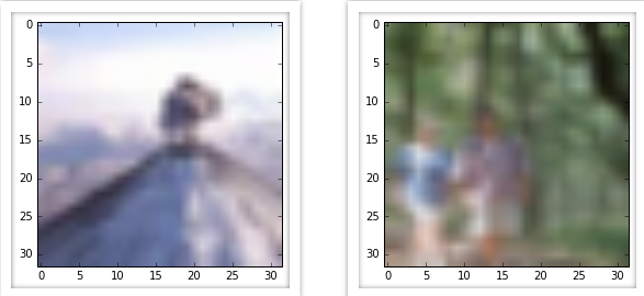
Figure 4. Few images from cifar test dataset
I trained it for 25 epoch and i got 35.96% test accuracy. you may go for higher epoch for higher accuracy.
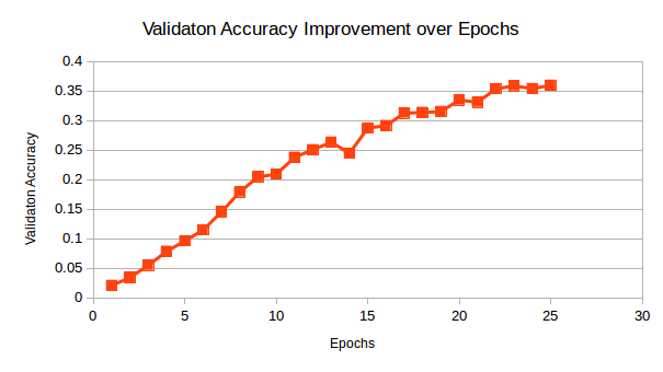
Figure. 5 Improvement in Accuracy with Epochs
Hope you could understand, how to play with images and ConvNet. In coming tutorial I will discuss all things in more details.


Comments